Neural Network Architectures

Deep neural networks and Deep Learning are powerful and popular algorithms. And a lot of their success lays in the careful design of the neural network architecture.

I wanted to revisit the history of neural network design in the last few years and in the context of Deep Learning.

For a more in-depth analysis and comparison of all the networks reported here, please see our recent article (and updated post). One representative figure from this article is here:

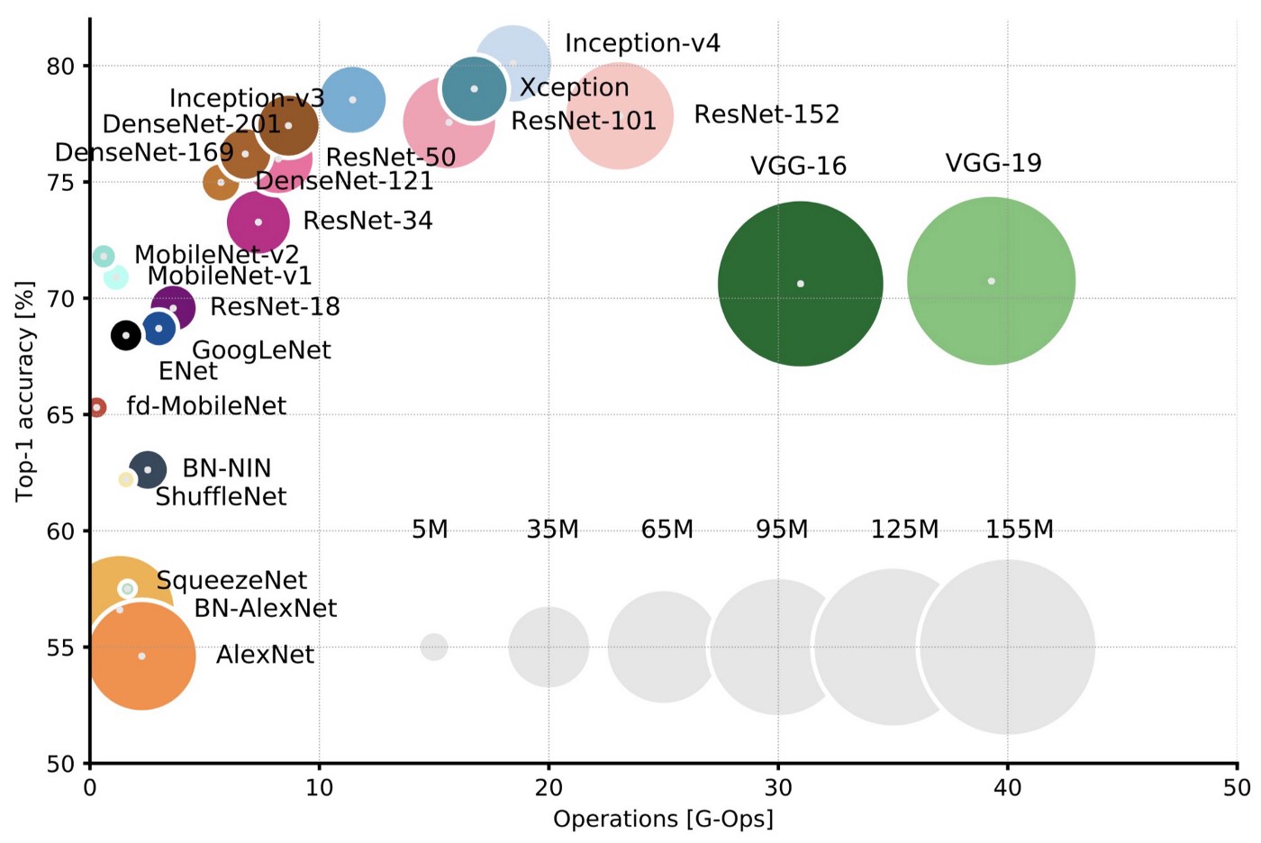
Top1 vs. operations, size ∝ parameters. Top-1 one-crop accuracy versus amount of operations required for a single forward pass. See also here

Reporting top-1 one-crop accuracy versus amount of operations required for a single forward pass in multiple popular neural network architectures.

LeNet5

It is the year 1994, and this is one of the very first convolutional neural networks, and what propelled the field of Deep Learning. This pioneering work by Yann LeCun was named LeNet5 after many previous successful iterations since the year 1988!

The LeNet5 architecture was fundamental, in particular the insight that image features are distributed across the entire image, and convolutions with learnable parameters are an effective way to extract similar features at multiple location with few parameters. At the time there was no GPU to help training, and even CPUs were slow. Therefore being able to save parameters and computation was a key advantage. This is in contrast to using each pixel as a separate input of a large multi-layer neural network. LeNet5 explained that those should not be used in the first layer, because images are highly spatially correlated, and using individual pixel of the image as separate input features would not take advantage of these correlations.

LeNet5 features can be summarized as:

• convolutional neural network use sequence of 3 layers: convolution,pooling, non-linearity –> This may be the key feature of Deep Learning for images since this paper!
• use convolution to extract spatial features
• subsample using spatial average of maps
• non-linearity in the form of tanh or sigmoids
• multi-layer neural network (MLP) as final classifier
• sparse connection matrix between layers to avoid large computational cost

In overall this network was the origin of much of the recent architectures, and a true inspiration for many people in the field.

The gap

In the years from 1998 to 2010 neural network were in incubation. Most people did not notice their increasing power, while many other researchers slowly progressed. More and more data was available because of the rise of cell-phone cameras and cheap digital cameras. And computing power was on the rise, CPUs were becoming faster, and GPUs became a general-purpose computing tool. Both of these trends made neural network progress, albeit at a slow rate. Both data and computing power made the tasks that neural networks tackled more and more interesting. And then it became clear…

Dan Ciresan Net

In 2010 Dan Claudiu Ciresan and Jurgen Schmidhuber published one of the very fist implementations of GPU Neural nets. This implementation had both forward and backward implemented on a a NVIDIA GTX 280 graphic processor of an up to 9 layers neural network.

AlexNet

In 2012, Alex Krizhevsky released AlexNet which was a deeper and much wider version of the LeNet and won by a large margin the difficult ImageNet competition.

AlexNet scaled the insights of LeNet into a much larger neural network that could be used to learn much more complex objects and object hierarchies.The contribution of this work were:

• use of rectified linear units (ReLU) as non-linearities
• use of dropout technique to selectively ignore single neurons during training, a way to avoid overfitting of the model
• overlapping max pooling, avoiding the averaging effects of average pooling
• use of GPUs NVIDIA GTX 580 to reduce training time

At the time GPU offered a much larger number of cores than CPUs, and allowed 10x faster training time, which in turn allowed to use larger datasets and also bigger images.

The success of AlexNet started a small revolution. Convolutional neural network were now the workhorse of Deep Learning, which became the new name for “large neural networks that can now solve useful tasks”.

Overfeat

In December 2013 the NYU lab from Yann LeCun came up with Overfeat, which is a derivative of AlexNet. The article also proposed learning bounding boxes, which later gave rise to many other papers on the same topic. I believe it is better to learn to segment objects rather than learn artificial bounding boxes.

VGG

The VGG networks from Oxford were the first to use much smaller 3×3 filters in each convolutional layers and also combined them as a sequence of convolutions.

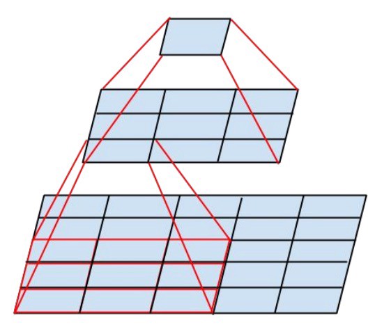
This seems to be contrary to the principles of LeNet, where large convolutionswere used to capture similar features in an image. Instead of the 9×9 or 11×11 filters of AlexNet, filters started to become smaller, too dangerously close to the infamous 1×1 convolutions that LeNet wanted to avoid, at least on the first layers of the network. But the great advantage of VGG was the insight that multiple 3×3 convolution in sequence can emulate the effect of larger receptive fields, for examples 5×5 and 7×7. These ideas will be also used in more recent network architectures as Inception and ResNet.

The VGG networks uses multiple 3x3 convolutional layers to represent complex features. Notice blocks 3, 4, 5 of VGG-E: 256×256 and 512×512 3×3 filters are used multiple times in sequence to extract more complex features and the combination of such features. This is effectively like having large 512×512 classifiers with 3 layers, which are convolutional! This obviously amounts to a massive number of parameters, and also learning power. But training of these network was difficult, and had to be split into smaller networks with layers added one by one. All this because of the lack of strong ways to regularize the model, or to somehow restrict the massive search space promoted by the large amount of parameters.

VGG used large feature sizes in many layers and thus inference was quite costly at run-time. Reducing the number of features, as done in Inception bottlenecks, will save some of the computational cost.

Network-in-network

Network-in-network (NiN) had the great and simple insight of using 1x1 convolutions to provide more combinational power to the features of a convolutional layers.

The NiN architecture used spatial MLP layers after each convolution, in order to better combine features before another layer. Again one can think the 1x1 convolutions are against the original principles of LeNet, but really they instead help to combine convolutional features in a better way, which is not possible by simply stacking more convolutional layers. This is different from using raw pixels as input to the next layer. Here 1×1 convolution are used to spatially combine features across features maps after convolution, so they effectively use very few parameters, shared across all pixels of these features!

The power of MLP can greatly increase the effectiveness of individual convolutional features by combining them into more complex groups. This idea will be later used in most recent architectures as ResNet and Inception and derivatives.

NiN also used an average pooling layer as part of the last classifier, another practice that will become common. This was done to average the response of the network to multiple are of the input image before classification.

GoogLeNet and Inception

Christian Szegedy from Google begun a quest aimed at reducing the computational burden of deep neural networks, and devised the GoogLeNet the first Inception architecture.

By now, Fall 2014, deep learning models were becoming extermely useful in categorizing the content of images and video frames. Most skeptics had given in that Deep Learning and neural nets came back to stay this time. Given the usefulness of these techniques, the internet giants like Google were very interested in efficient and large deployments of architectures on their server farms.

Christian thought a lot about ways to reduce the computational burden ofdeep neural nets while obtaining state-of-art performance (on ImageNet, for example). Or be able to keep the computational cost the same, while offering improved performance.

He and his team came up with the Inception module:

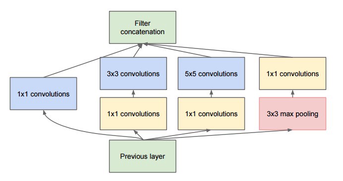
which at a first glance is basically the parallel combination of 1×1, 3×3, and 5×5 convolutional filters. But the great insight of the inception module was the use of 1×1 convolutional blocks (NiN) to reduce the number of features before the expensive parallel blocks. This is commonly referred as “bottleneck”. This deserves its own section to explain: see “bottleneck layer” section below.

GoogLeNet used a stem without inception modules as initial layers, and an average pooling plus softmax classifier similar to NiN. This classifier is also extremely low number of operations, compared to the ones of AlexNet and VGG. This also contributed to a very efficient network design.

Bottleneck layer

Inspired by NiN, the bottleneck layer of Inception was reducing the number of features, and thus operations, at each layer, so the inference time could be kept low. Before passing data to the expensive convolution modules, the number of features was reduce by, say, 4 times. This led to large savings in computational cost, and the success of this architecture.

Let’s examine this in detail. Let’s say you have 256 features coming in, and 256 coming out, and let’s say the Inception layer only performs 3x3 convolutions. That is 256x256 x 3x3 convolutions that have to be performed (589,000s multiply-accumulate, or MAC operations). That may be more than the computational budget we have, say, to run this layer in 0.5 milli-seconds on a Google Server. Instead of doing this, we decide to reduce the number of features that will have to be convolved, say to 64 or 256/4. In this case, we first perform 256 -> 64 1×1 convolutions, then 64 convolution on all Inception branches, and then we use again a 1x1 convolution from 64 -> 256 features back again. The operations are now:

• 256×64 × 1×1 = 16,000s
• 64×64 × 3×3 = 36,000s
• 64×256 × 1×1 = 16,000s

For a total of about 70,000 versus the almost 600,000 we had before. Almost 10x less operations!

And although we are doing less operations, we are not losing generality in this layer. In fact the bottleneck layers have been proven to perform at state-of-art on the ImageNet dataset, for example, and will be also used in later architectures such as ResNet.

The reason for the success is that the input features are correlated, and thus redundancy can be removed by combining them appropriately with the 1x1 convolutions. Then, after convolution with a smaller number of features, they can be expanded again into meaningful combination for the next layer.

Inception V3 (and V2)

Christian and his team are very efficient researchers. In February 2015 Batch-normalized Inception was introduced as Inception V2. Batch-normalizationcomputes the mean and standard-deviation of all feature maps at the output of a layer, and normalizes their responses with these values. This corresponds to “whitening” the data, and thus making all the neural maps have responses in the same range, and with zero mean. This helps training as the next layer does not have to learn offsets in the input data, and can focus on how to best combine features.

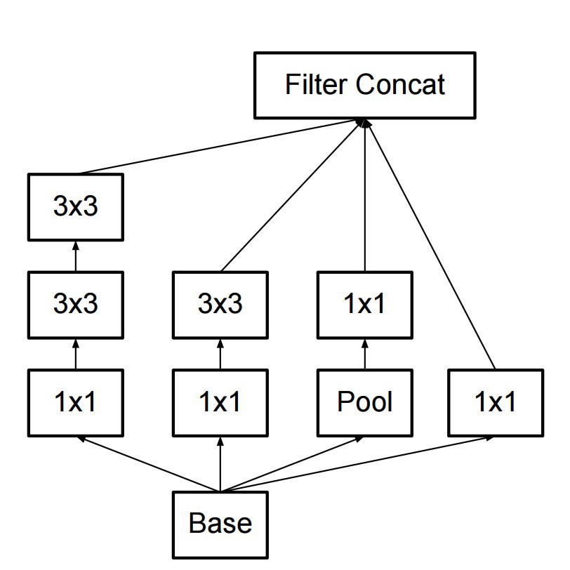
In December 2015 they released a new version of the Inception modules and the corresponding architecture This article better explains the original GoogLeNet architecture, giving a lot more detail on the design choices. A list of the original ideas are:

• maximize information flow into the network, by carefully constructing networks that balance depth and width. Before each pooling, increase the feature maps.
• when depth is increased, the number of features, or width of the layer is also increased systematically
• use width increase at each layer to increase the combination of features before next layer
• use only 3x3 convolution, when possible, given that filter of 5x5 and 7x7can be decomposed with multiple 3x3. See figure:

• the new inception module thus becomes:

• filters can also be decomposed by flattened convolutions into more complex modules:

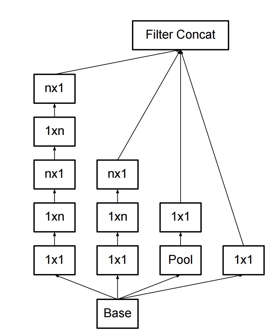
• inception modules can also decrease the size of the data by providing pooling while performing the inception computation. This is basically identical to performing a convolution with strides in parallel with a simple pooling layer:

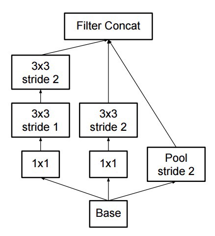
Inception still uses a pooling layer plus softmax as final classifier.

ResNet

The revolution then came in December 2015, at about the same time as Inception v3. ResNet have a simple ideas: feed the output of two successive convolutional layer AND also bypass the input to the next layers!

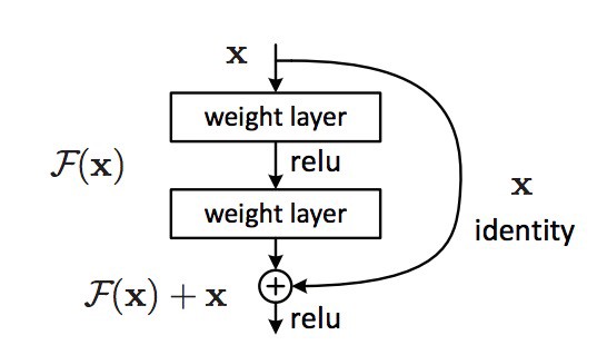
This is similar to older ideas like this one. But here they bypass TWO layers and are applied to large scales. Bypassing after 2 layers is a key intuition, as bypassing a single layer did not give much improvements. By 2 layers can be thought as a small classifier, or a Network-In-Network!

This is also the very first time that a network of > hundred, even 1000 layers was trained.

ResNet with a large number of layers started to use a bottleneck layer similar to the Inception bottleneck:

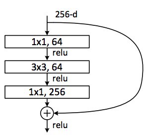
This layer reduces the number of features at each layer by first using a 1x1 convolution with a smaller output (usually 1/4 of the input), and then a 3x3 layer, and then again a 1x1 convolution to a larger number of features. Like in the case of Inception modules, this allows to keep the computation low, while providing rich combination of features. See “bottleneck layer” section after “GoogLeNet and Inception”.

ResNet uses a fairly simple initial layers at the input (stem): a 7x7 conv layer followed with a pool of 2. Contrast this to more complex and less intuitive stems as in Inception V3, V4.

ResNet also uses a pooling layer plus softmax as final classifier.

Additional insights about the ResNet architecture are appearing every day:

• ResNet can be seen as both parallel and serial modules, by just thinking of the inout as going to many modules in parallel, while the output of each modules connect in series
• ResNet can also be thought as multiple ensembles of parallel or serial modules
• it has been found that ResNet usually operates on blocks of relatively low depth ~20–30 layers, which act in parallel, rather than serially flow the entire length of the network.
• ResNet, when the output is fed back to the input, as in RNN, the network can be seen as a better bio-plausible model of the cortex

Inception V4

And Christian and team are at it again with a new version of Inception.

The Inception module after the stem is rather similar to Inception V3:

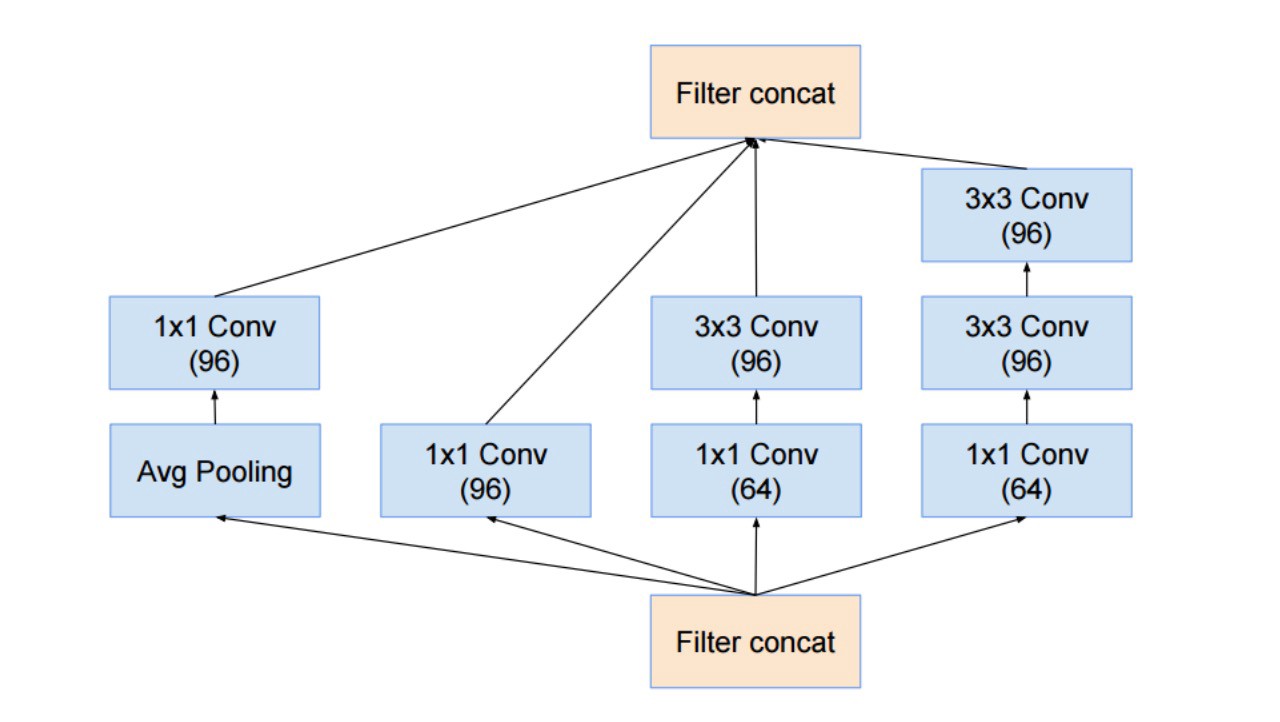
They also combined the Inception module with the ResNet module:

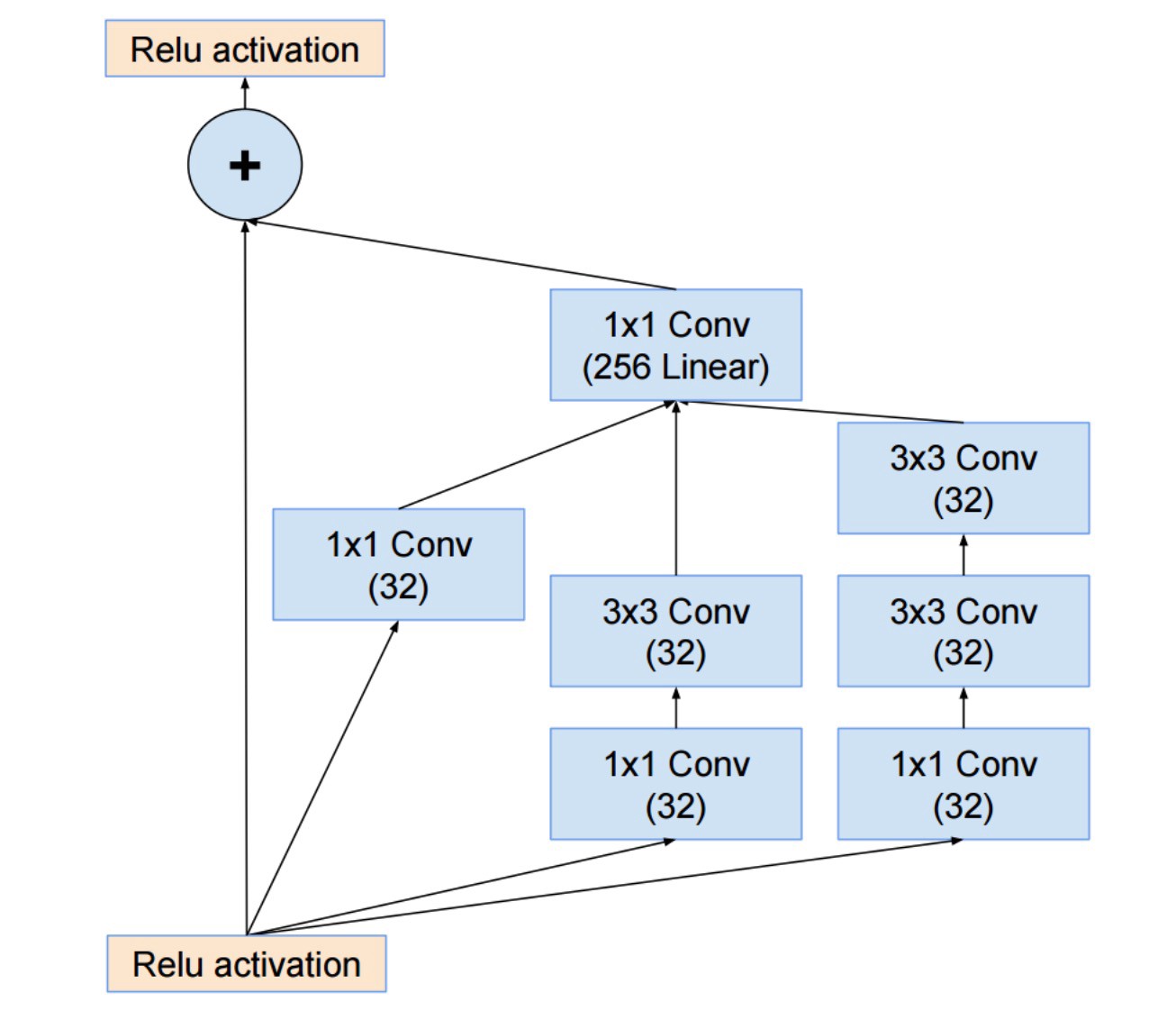
This time though the solution is, in my opinion, less elegant and more complex, but also full of less transparent heuristics. It is hard to understand the choices and it is also hard for the authors to justify them.

In this regard the prize for a clean and simple network that can be easily understood and modified now goes to ResNet.

SqueezeNet

SqueezeNet has been recently released. It is a re-hash of many concepts from ResNet and Inception, and show that after all, a better design of architecture will deliver small network sizes and parameters without needing complex compression algorithms.

ENet

Our team set up to combine all the features of the recent architectures into a very efficient and light-weight network that uses very few parameters and computation to achieve state-of-the-art results. This network architecture is dubbed ENet, and was designed by Adam Paszke. We have used it to perform pixel-wise labeling and scene-parsing. Here are some videos of ENet in action. These videos are not part of the training dataset.

The technical report on ENet is available here. ENet is a encoder plus decoder network. The encoder is a regular CNN design for categorization, while the decoder is a upsampling network designed to propagate the categories back into the original image size for segmentation. This worked used only neural networks, and no other algorithm to perform image segmentation.

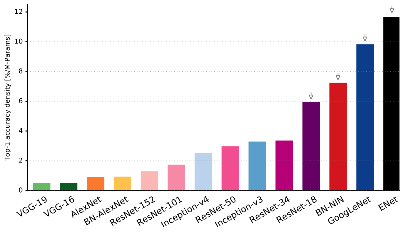
As you can see in this figure ENet has the highest accuracy per parameter used of any neural network out there!

ENet was designed to use the minimum number of resources possible from the start. As such it achieves such a small footprint that both encoder and decoder network together only occupies 0.7 MB with fp16 precision. Even at this small size, ENet is similar or above other pure neural network solutions in accuracy of segmentation.

An analysis of modules

A systematic evaluation of CNN modules has been presented. The found out that is advantageous to use:

• use ELU non-linearity without batchnorm or ReLU with it.

• apply a learned colorspace transformation of RGB.

• use the linear learning rate decay policy.

• use a sum of the average and max pooling layers.

• use mini-batch size around 128 or 256. If this is too big for your GPU, decrease the learning rate proportionally to the batch size.

• use fully-connected layers as convolutional and average the predictions for the final decision.

• when investing in increasing training set size, check if a plateau has not been reach. • cleanliness of the data is more important then the size.

• if you cannot increase the input image size, reduce the stride in the con- sequent layers, it has roughly the same effect.

• if your network has a complex and highly optimized architecture, like e.g. GoogLeNet, be careful with modifications.

Xception

Xception improves on the inception module and architecture with a simple and more elegant architecture that is as effective as ResNet and Inception V4.

The Xception module is presented here:

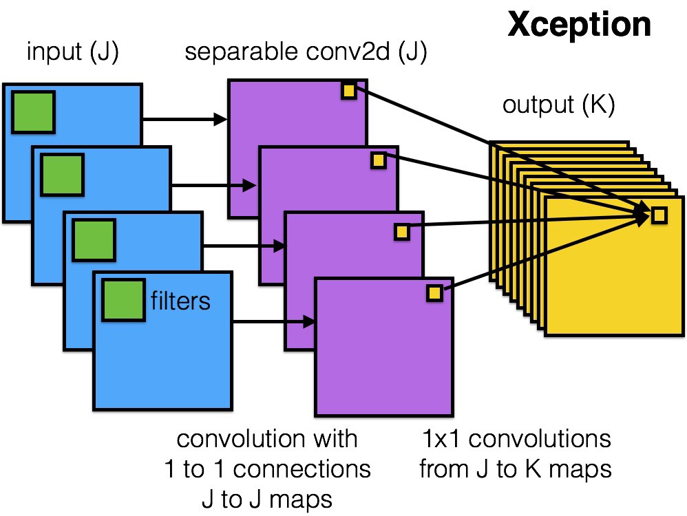
This network can be anyone’s favorite given the simplicity and elegance of the architecture, presented here:

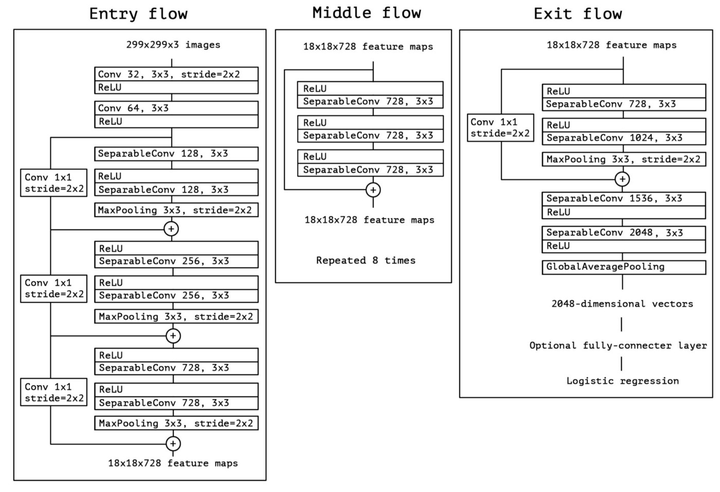
The architecture has 36 convolutional stages, making it close in similarity to a ResNet-34. But the model and code is as simple as ResNet and much more comprehensible than Inception V4.

A Torch7 implementation of this network is available here An implementation in Keras/TF is availble here.

It is interesting to note that the recent Xception architecture was also inspired by our work on separable convolutional filters.

MobileNets

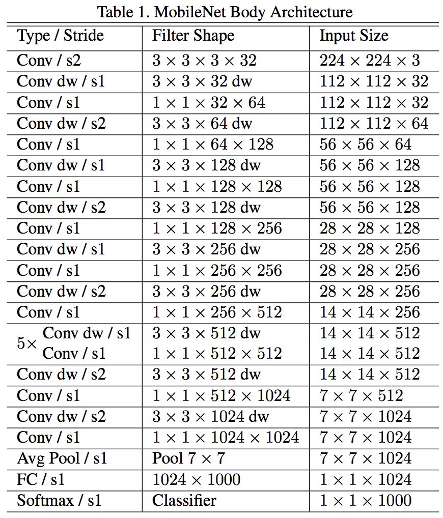
A new MobileNets architecture is also available since April 2017. This architecture uses separable convolutions to reduce the number of parameters. The separate convolution is the same as Xception above. Now the claim of the paper is that there is a great reduction in parameters — about 1/2 in case of FaceNet, as reported in the paper. Here is the complete model architecture:

MobileNets

Unfortunately, we have tested this network in actual application and found it to be abysmally slow on a batch of 1 on a Titan Xp GPU. Look at a comparison here of inference time per image:

• resnet18 : 0.002871
• alexnet : 0.001003
• vgg16 : 0.001698
• squeezenet : 0.002725
• mobilenet : 0.033251

Clearly this is not a contender in fast inference! It may reduce the parameters and size of network on disk, but is not usable.

Other notable architectures

FractalNet uses a recursive architecture, that was not tested on ImageNet, and is a derivative or the more general ResNet.

Update

For an update on comparison, please see this post.

The future

We believe that crafting neural network architectures is of paramount importance for the progress of the Deep Learning field. Our group highly recommends reading carefully and understanding all the papers in this post.

But one could now wonder why we have to spend so much time in crafting architectures, and why instead we do not use data to tell us what to use, and how to combine modules. This would be nice, but now it is work in progress. Some initial interesting results are here.

Note also that here we mostly talked about architectures for computer vision. Similarly neural network architectures developed in other areas, and it is interesting to study the evolution of architectures for all other tasks also.

If you are interested in a comparison of neural network architecture and computational performance, see our recent paper.

Acknowledgments

This post was inspired by discussions with Abhishek Chaurasia, Adam Paszke, Sangpil Kim, Alfredo Canziani and others in our e-Lab at Purdue University.

About the author

I have almost 20 years of experience in neural networks in both hardware and software (a rare combination). See about me here: Medium, webpage, Scholar, LinkedIn, and more…