Computation and memory bandwidth in deep neural networks

Eugenio Culurciello, Aliasger Zaidy and Vinayak Gokhale

Memory bandwidth and data re-use in deep neural network computation can be estimated with a few simple simulations and calculations.

Deep neural network computation requires the use of weight data and _input_data. Weights are neural network parameters, and input data (maps, activations) is the data you want to process from one layer to the next.

In general, if a computation re-uses data, it will require less memory bandwidth. Re-use can be accomplished by:

• sending more inputs to be processed by the same weights
• sending more weights to process the same inputs

If there is no input or weight data re-use, then the bandwidth is at a maximum for a given application. Let us give some examples:

Linear layers: here a weight matrix of M by M is used to process a vector of M values with b bits. Total data transferred is: b(M+M²) or ~bM²

If the linear layer is used only for one vector, it will require to send the entire M² matrix of weights as computation occurs. If your system has T_operations/second of performance, then the time to perform the computation is _bM²/T. Given than bandwidth BW = total data transferred / tim__e, in case of linear layers BW = T.

This means that if your system has 128 G-ops/s of performance, you will need a bandwidth of more than 128 GB/s to perform the operation at full system efficiency (provided, of course that the system can do this!).

Of course if you have multiple inputs for the same linear layer (multiple vectors that need to be multiplied by the same matrix) then: BW = T/B, where B is the number of vectors or Batch.

Convolutions: for convolution operation, the bandwidth requirements are usually lower, as an input map data can be used in several convolution operation in parallel, and convolution weights are relatively small.

For example: a 13 x 13 pixel map in a 3x3 convolution operation from 192 input maps to 192 output maps (as, for example, in Alexnet layer 3) requires: ~4MB weight data and ~0.1MB input data from memory. This may require about 3.2 GB/s to be performed on a 128 G-ops/s system with ~99% efficiency (SnowFlake Spring 2017 version). The bandwidth usage is low is because the same input data is used to compute 192 outputs, albeit with different small weight matrices.

RNN: memory bandwidth for recurrent neural networks is one of the highest. Deep Speech 2 system or similar use 4 RNN layers of 400 size (see here and here). Each layer uses the equivalent of 3 linear-layer-like matrix multiplications in a GRU model. During inference the input batch is only 1 or a small number, and thus running these neural network requires the highest amount of memory bandwidth, so high it usually it is not possible to fully utilize even efficient hardware at full utilization.

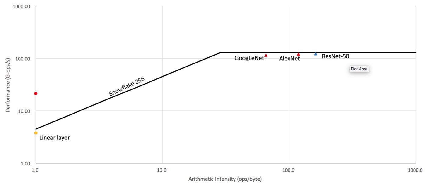
In order to visualize these concepts, refer to this figure:

Snowflake arithmetic intensity

This is the arithmetic intensity for our accelerator Snowflake. Arithmetic intensity is the number of operations performed on a byte of data. As you can see all neural network models tested perform at the maximum (roofline) efficiency of the device. On the other hand linear layers have very little data re-use and are limited by memory bandwidth constraints.

PS.: More about performance, roofline-plots and bandwidth here.

About the author

I have almost 20 years of experience in neural networks in both hardware and software (a rare combination). See about me here: Medium, webpage, Scholar, LinkedIn, and more…